Vibrational frequencies

A frequency calculation can be performed either numerically or analytically. The numerical approach is implemented directly in ASH and can always be applied to any QM, MM or QM/MM theory (requires the method to have an analytical gradient, however) while the analytical approach is only available if the QM program contains the functionality and if the ASH interface to that theory supports it (see below)

For QM/MM Hamiltonians, the numerical approach is the only available option.

Numerical frequencies

Numerical frequencies can be performed with ASH using any QM, MM or QM/MM theory object. A QM-method that has available an analytical gradient (i.e. 1st derivative of energy) in the external code should typically be used. Most HF, DFT, MP2 and CASSCF methods have analytical gradients implemented in QM codes.

Note that a numerical 2nd derivative on top of a numerical 1st derivative can in principle be done but is not recommended (accumulation of numerical noise).

Use the NumFreq function to request a numerical frequency job. The function requires a fragment object and a theory level at minimum. The fragment object should typically contain a fragment with optimized coordinates at same level of theory (i.e. an already optimized minimum or saddlepoint).

def NumFreq(fragment=None, theory=None, npoint=2, displacement=0.005, hessatoms=None, numcores=1, runmode='serial',
        temp=298.15, pressure=1.0, hessatoms_masses=None, printlevel=1, charge=None, mult=None):

Keyword	Type	Default value	Details
`fragment`	ASH Fragment	None	ASH Fragment object.
`theory`	ASHTheory object	None	ASH Theory object.
`runmode`	String	'serial	Whether to run the numerical frequency displacement calculations in serial (sequentially) or in parallel using Python multiprocessing.
`npoint`	Integer	2	Whether to do a 1-point or 2-point approximation for the Hessian. 1-point takes half as many displacements as 2-point and is less accurate.
`displacement`	Float	0.005	Size of displacement (in Å) to take.
`hessatoms`	list	None	Optional list of atom indices that will be displaced and define a partial Hessian instead of a full Hessian. If None, all atoms in Fragment will be displaced.
`temp`	Float	298.15	Temperature (in K) to use in thermochemistry calculation.
`pressure`	Float	1.0	Pressure (in atm) to use in thermochemistry calculation.
`hessatoms_masses`	list	None	Optional list of masses for the Hessian atoms.
`charge`	integer	None	Optional charge. Will override charge attribute of ASH Fragment.
`mult`	integer	None	Optional spin multiplicity. Will override mult attribute of ASH Fragment.
`printlevel`	integer	1	The printlevel.

1-point vs. 2-point Hessian

Additionally you can select to do a 1-point Hessian or a 2-point Hessian by the npoint keyword (value of 1 or 2). A 1-point Hessian makes a single displacement (+ direction) for each atom and each x,y and z-coordinate from the input geometry. This option is reasonably accurate and is the default. A more accurate 2-point Hessian makes displacement in both + and - directions (for each x-, y- and z-coordinate of each atom), is twice as expensive (double the displacements) but is more accurate. The displacement step can be changed if required. The default recommended setting is: 0.0005 Å.

Serial or parallel calculation

Two runmodes are available: 'serial' and 'parallel'.

Serial

The default 'serial' mode will run each displacement sequentially. The Energy+Gradient calculation of each displacment can, however, still be parallelized if the QM or QM/MM object has this information available. For example if an ORCATheory object has been defined with numcores=8 then ORCA will run each Energy+Gradient evaluation with 8 cores using the OpenMPI parallelization of ORCA.

Parallel

For numerical frequencies, it is usually much more efficient, however, to run the displacement jobs simultaneously in parallel fashion. This is accomplished using runmode='parallel' and the parallelization will be linear scaling (almost always recommended). As there are almost always many more displacements available than CPUs, the parallelization of the QM or QM/MM object should usually be turned off and instead as many displacements are run simultaneously as there are number of cores. For example, for a 30-atom system, there are 90 XYZ coordinates. For a 2-point Hessian, this means that 180 displacements to be calculated. If 20 cores are available, then 20 displacements can be run simultaneously, fully utilizing all 20 cores. This will require 9 runs in total (20*9=180).

Warning

Parallel runmode is currently not available for QM/MM calculations.

Full or partial Hessian

A partial Hessian can be easily performed instead of the full Hessian. This is an excellent approximation for vibrational modes with rather local character and the quality of the approximation can be controlled.

For a QM/MM model of a protein active site with a common active region of about 1000 atoms, the full Hessian of all 1000 atoms would actually not be a doable or recommended calculation. Instead a partial Hessian job of the important atoms (e.g. the QM region) makes more sense.

A partial Hessian job is performed if a list of Hessian atoms (e.g. hessatoms=[0,1,2] ) is passed to the NumFreq function. In this case, the displacements will only be calculated for the list of "hessatoms" and the result is a partial Hessian for the chosen atoms of the system.

Final output

Once the displacements are complete, the gradients for all displacements are combined to give the full (or partial) Hessian. The Hessian is mass-weighted and diagonalized which results in the harmonic vibrational frequencies as eigenvalues and the normal modes as eigenvectors. Rotational and translational modes are projected out if the full Hessian is calculated.

An elemental normal mode composition factor analysis is automatically performed on the modes and thermochemistry based on the rigid-rotor-harmonic-oscillator (RRHO) approximation with a default temperature and pressure of 298 K and 1 atm.

Upon completion of the job, the full Hessian can be accessed in a few different ways:

It is stored in the hessian attribute of the ASH_Results object returned from the NumFreq function (see example below).
It is present in a file named "Hessian" in the "Numfreq_dir" (created by ASH). Can be read back into ASH using the read_hessian function.
It is present in an ORCA_formatted Hessian-file named "orcahessfile.hess". Can be read back into ASH using read_ORCA_Hessian

Additionally ASH creates a file "orcahessfile.hess_dummy.out" which is a dummy ORCA output file that contains the frequencies and normal modes. This file can be conveniently opened by some visualization programs such as Chemcraft and allows you to visualize the normal modes.

Examples:

Numerical frequencies in serial mode (QM-code parallelization instead used):

from ash import *

#the total number of CPU cores available to Ash (should match the job-script)
numcores=8

frag=Fragment(xyzfile="h2o.xyz", charge=0, mult=1)

#ORCA theory object, ORCA parallelization turned off by not providing numcores keyword
ORCAcalc = ORCATheory(orcasimpleinput="! r2SCAN-3c tightscf", numcores=numcores)

#Serial Numfreq job (default):
freqresult = NumFreq(fragment=frag, theory=ORCAcalc, npoint=2, runmode='serial')

print("freqresult:", freqresult)
#Print Hessian
print("Hessian:", freqresult.hessian)

The resulting object from a NumFreq calculation is an ASH_Results dataclass object. It contains the calculated frequencies, eigenvectors, normalmodes, list-of frequencies and a dictionary of thermochemical properties.

Numerical frequencies in parallel mode (QM-code parallelization turned off):

from ash import *

#the total number of CPU cores available to Ash (should match the job-script)
numcores=8

frag=Fragment(xyzfile="h2o.xyz", charge=0, mult=1)

#ORCA theory object, ORCA parallelization turned off by not providing numcores keyword
ORCAcalc = ORCATheory(orcasimpleinput="! r2SCAN-3c tightscf")

#Parallel mode: ASH will use the number of cores given to run same number of displacments simultaneously.
freqresult = NumFreq(fragment=frag, theory=ORCAcalc, npoint=2, runmode='parallel', numcores=numcores)

print("Vibrational frequencies (cm**-1) : ", freqresult['frequencies'])
print("ZPVE (Eh) : ", freqresult['ZPVE'])
print("Gibbs energy corrections (Eh) : ", freqresult['Gcorr'])

Analytical frequencies

Some QM programs have analytical frequencies implemented and the ASH interface may support requesting the calculation of the analytical Hessian and reading Hessian back. Currently analytical frequencies are only supported in the QM codes: ORCATheory and CFourTheory

An analytical Hessian calculation is requested by the AnFreq function that takes fragment and theory as necessary arguments:

def AnFreq(fragment=None, theory=None, numcores=1, temp=298.15, pressure=1.0)

Example:

HF_frag=Fragment(xyzfile="hf.xyz")
ORCAcalc = ORCATheory(orcasimpleinput='BP86 def2-SVP def2/J tightscf', orcablocks="", numcores=1)
freqresult = AnFreq(theory=ORCAcalc, fragment=HF_frag)

print("Thermochem properties dict:", freqresult.thermochemistry)
print("Vibrational frequencies (cm**-1) : ", freqresult.frequencies)

thermochemistry corrections

Thermochemistry corrections are automatically calculated when either a Numfreq or Anfreq job is requested.

result_anfreq = AnFreq(theory=ORCAcalc, fragment=HF_frag)
result_numfreq = NumFreq(theory=ORCAcalc, fragment=HF_frag)

print("Thermochem property dict:", result_numfreq.thermochemistry)
print("ZPVE (Eh) : ", result_numfreq.thermochemistry['ZPVE'])
print("Gibbs energy corrections (Eh) : ", result_numfreq.thermochemistry['Gcorr'])

The return object from AnFreq or NumFreq contains a thermochemistry dictionary that contains the following information as dictionary keys. Note that the entropy terms (TS) are in energy units (Eh) as they have been multiplied by temperature T.

Key	Property
frequencies	The harmonic vibrational frequencies (list).
ZPVE	Zero-point vibrational energy (harmonic)
E_trans	Translational energy at temp T.
E_rot	Translational energy at temp T.
E_vib	Vibrational energy at temp T.
E_tot	Total energy at temp T.
TS_trans	Translational entropy at temp T (in energy units).
TS_rot	Rotational entropy at temp T (in energy units)
TS_vib	Vibrational entropy at temp T (in energy units)
TS_el	Electronic entropy at temp T (in energy units)
TS_tot	Total entropy at temp T (in energy units)
vibenergycorr	Vibrational energy correction at temp T.
Hcorr	Total enthalpy correction at temp T.
Gcorr	Gibbs free energy correction at temp T.

Alternatively, the thermochemcalc function can be called directly.

def thermochemcalc(vfreq,atoms,fragment, multiplicity, temp=298.18,pressure=1.0):

This function calculates the thermodynamic corrections from a list of available frequencies, number of atoms, ASH fragment object and spin multiplicity. The temperature (default: 298.15 K) and pressure (default: 1.0 atm) can be specified.

h2o_frag = Fragment(xyzfile="h2o.xyz")
#Manually defined frequencies for system
frequencies=[1600.1, 2300.2, 2400.3]
thermochemcalc(frequencies,3,h2o_frag, 1, temp=298.18, pressure=1.0)

Calculating IR and Raman spectra

Calculation of IR and Raman spectra requires either the dipole derivatives or the polarizability derivatives along the normal modes. This means that to get IR/Raman intensitites from a numerical frequency calculation the dipole moment (IR) or polarizability (Raman) must be calculated for each displacement by the QM-code.

IR/Raman spectra can be calculated for any QM-level of theory for which analytical gradients (first derivatives) are available and if dipole moments/polarizabilities are available in the code or supported by ASH interface (see below). QM/MM theories within ASH are also supported.

IR intensities:

In the ASH interfaces to ORCA, pySCF, xTB, MRCC, CFour, Block and Dice, the dipole moments are automatically available and the NumFreq module will in this case get the dipole moment from each calculation and automatically calculate the dipole derivatives along the normal modes and provide the final IR intensity for each normal mode. The IR intensities are stored in the ASH_Results object returned from the NumFreq function.

Example: IR intensities using ORCA

from ash import *

frag=Fragment(databasefile="h2o.xyz", charge=0, mult=1)

#ORCA theory
ORCAcalc = ORCATheory(orcasimpleinput="! r2SCAN-3c tightscf", numcores=4)

#Serial Numfreq job
result = NumFreq(fragment=frag, theory=ORCAcalc, npoint=2, runmode='serial')

print("Vibrational frequencies (cm**-1) : ", result.frequencies)
print("IR intensities (km/mol): ", result.IR_intensities)

Raman activities:

Raman activities are a bit more complicated. Analytic polarizabilities are not always available in the QM-code and they are much more expensive. Polarizabilities are available in the ASH interface to ORCA, pySCF and CFour. To get the Raman activities one must i) tell the QM-code to calculate polarizabilities and ii) tell the NumFreq module that one wants Raman (Raman=True).

Example: Raman activities using ORCA

from ash import *

frag=Fragment(databasefile="h2o.xyz", charge=0, mult=1)

# ORCA Theory requesting polarizability calculation
blocks="""
%elprop
polar 1
end
"""
ORCAcalc = ORCATheory(orcasimpleinput="! r2SCAN-3c tightscf", orcablocks=blocks, numcores=4)

#NumFreq
result = NumFreq(fragment=frag, theory=ORCAcalc, npoint=2, runmode='serial', Raman=True)

print("Vibrational frequencies (cm**-1) : ", result.frequencies)
print("Raman activities (Å^4/amu): ", result.Raman_activities)

Plot IR/Raman spectra:

The vibrational frequencies, IR intensities and Raman activitites can be found in the ASH output:

----------------------------------------
VIBRATIONAL FREQUENCY SUMMARY
----------------------------------------
Note: imaginary modes shown as negative
  Mode    Freq(cm**-1)   IR Int.(km/mol)  Raman Act.(Å^4/amu)
  0             0.0000        0.0000          0.0000            (TR mode)
  1             0.0000        0.0000          0.0000            (TR mode)
  2             0.0000        0.0000          0.0000            (TR mode)
  3             0.0000        0.0000          0.0000            (TR mode)
  4             0.0000        0.0000          0.0000            (TR mode)
  5             0.0000        0.0000          0.0000            (TR mode)
  6          1608.3146       81.7550          1.3155
  7          3851.9971        4.3099         74.7428
  8          3993.9783       63.5039         22.0644

and can also be found in the ASH Results object. If one wants to plot a broadened IR/Raman spectra one can use plot_Spectrum function (see Plotting), providing the frequencies and intensities from the Results object as x- and y-values.

from ash import *

frag=Fragment(databasefile="acetone.xyz", charge=0, mult=1)

#ORCA theory object
ORCAcalc = ORCATheory(orcasimpleinput="! r2SCAN-3c", numcores=4)

#Optimization
Optimizer(fragment=frag, theory=ORCAcalc)
#Frequencies
result = NumFreq(fragment=frag, theory=ORCAcalc, npoint=2, runmode='serial')

print("Vibrational frequencies (cm**-1) : ", result.frequencies)
print("IR intensities (km/mol): ", result.IR_intensities)

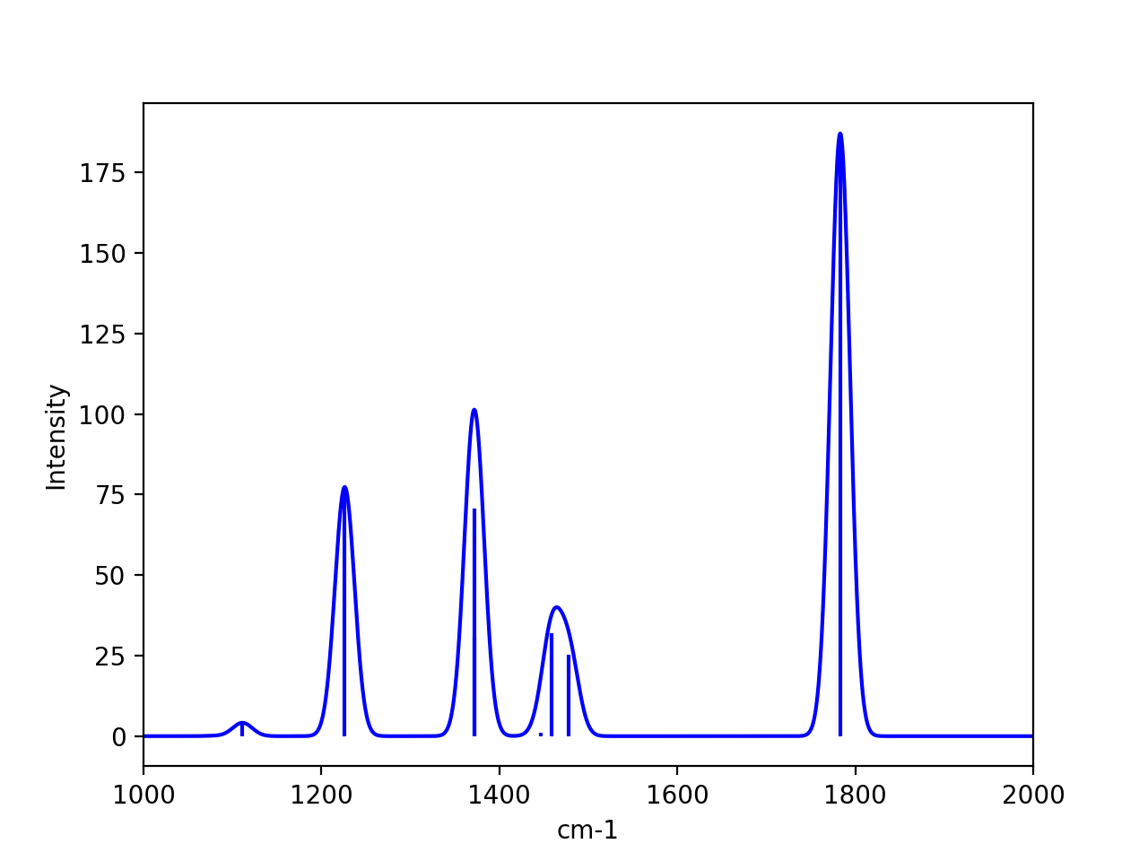
#Plotting broadened IR spectrum (11 cm-1 broadening, 5000 points) for 1000-2000 cm-1 window.
plot_Spectrum(xvalues=result.frequencies, yvalues=result.IR_intensities, plotname='IR_spectrum', range=[1000,2000], unit='cm-1',
    broadening=11, points=5000, imageformat='png', dpi=200)