PES: PhotoElectron/PhotoEmission Spectrum
Workflow to calculate photoelectron/photoemission spectra of molecules using a few different approaches: TDDFT, OODFT, CASSCF, MRCI or EOM-IP-CCSD state energies. Currently only ORCA is supported as QM-code. A Dyson-orbital norm approach via Wfoverlap program is used for intensities.
The OODFT workflow performs SCF calculations of all states utilizing the OODFT/deltaSCF approach as implemented in ORCA:
The TDDFT workflow combines an SCF-calculation of the initial state and an SCF+TDDFT calculation of the first ionized state (of each ionized-state multiplicity) to get the full ionization energy spectrum for each spin multiplicity. Dyson orbital norms are then calculated as approximate intensities for both SCF-type and TDDFT-type states by parsing theORCA TDDFT output files.
The CASSCF workflow performs a CASSCF calculation of the initial state and the uses the initial-state orbitals in a CAS-CI calculation of the ionized states of both spin multiplicities. Both regular CASSCF and ICE-CASSCF in ORCA is possible.
The MRCI workflow is similar to the CASSCF workflow but on top of the CASSCF orbital optimization of the initial state an MRCI calculation is performed and for the ionized state the initial-state orbitals are used as before. For CASSCF and MRCI, determinant-printing of the wavefunction is requested (printed in the output) which is parsed by the code and fed to the Wfoverlap program.
The IP-EOM-CCSD approach calculates the ionized states directly via the IP-EOM approach from the CCSD wavefunction of the initial state. Approximate Dyson norms are used here, i.e. the dominant coefficient of the singles eigenvector.
Notes:
ORCA is the only supported QM-code for now.
Intensities require the Wfoverlap program to calculate Dyson orbital norms via determinant-based wavefunctions.
Plotting option requires installation of Matplotlib.
Potential issues: Wfoverlap binary requires libblas.so.3 and liblapack.so.3 binaries. Make sure a directory containing these libraries is in your LD_LIBRARY_PATH.
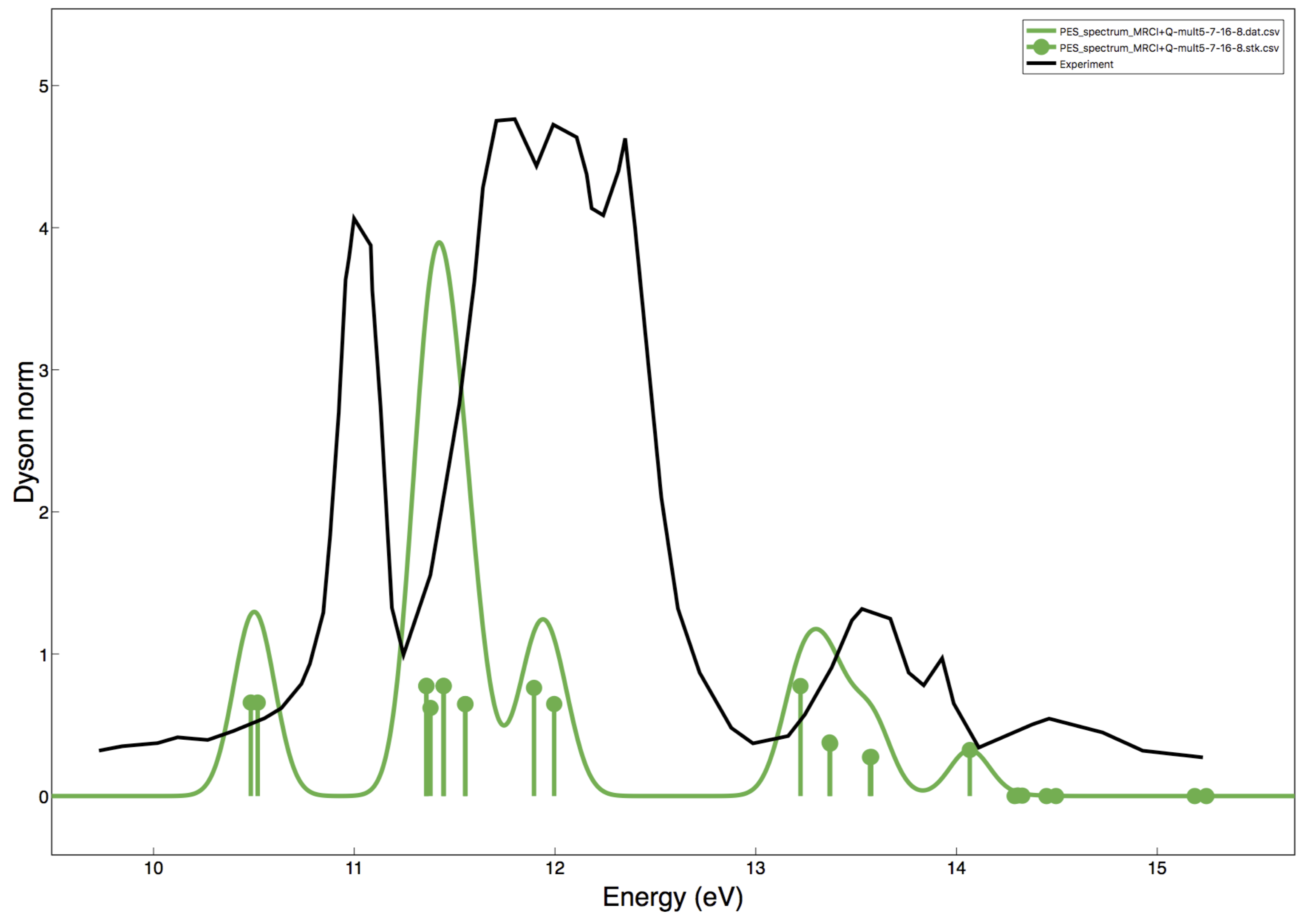
Figure 1. PES-spectrum via MRCI using ASH and ORCA
PhotoElectron function
def PhotoElectron(theory=None, fragment=None, method=None, vibrational_option=None, trajectory=None,
                        numcores=1, memory=40000,label=None,
                        Initialstate_charge=None, Initialstate_mult=None,
                        Ionizedstate_charge=None, Ionizedstate_mult=None, numionstates=5,
                        initialorbitalfiles=None, densities='None', densgridvalue=40,
                        deltaSCF_ionize=False, deltaSCF_PMOM=False, deltaSCFkeyword=None,
                        tda=True,brokensym=False, HSmult=None, atomstoflip=None, check_stability=True,
                        CAS_Initial=None, CAS_Final = None,
                        CASCI_Final=False,
                        MRCI_CASCI_Final=False, MRCI_SOC=False,
                        btPNO=False, DLPNO=False, no_shakeup=False, virt_offset=0,
                        path_wfoverlap=None, tprintwfvalue=1e-5, noDyson=False,
                        OODFT_CC=False)
How to use
The PhotoElectron function takes the following keyword arguments:
Necessary:
method: Options are "TDDFT", "OODFT", "EOM", "CAS-CI", "CASSCF", "NEVPT2", "NEVPT2-F12" "MRCI", "MREOM"
theory: An ASH Theory object (only ORCATheory supported at the moment)
fragment: An ASH fragment object
Initialstate_charge : integer
Initialstate_mult : integer
Ionizedstate_charge: integer
Ionizedstate_mult: integer or list of integers, e.g. [5,7]
path_wfoverlap: string
numionstates : integer (default: 50)
Optional:
memory: integer (in MB), (memory used by Wfoverlap, default: 40000)
numcores: integer (number of cores used in WFOverlap, default: 1) Note: ORCA parallelization is handled by ORCA object.
noDyson : Boolean(True/False), (whether to skip Dyson-norm computation, default: False)
tda : Boolean (default: True)
brokensym: Boolean (default: False)
HSmult : integer (for brokensym feature, default: None)
atomstoflip : list of integers (for brokensym feature, default: None)
initialorbitalfiles : list of filename-strings (for reading in orbital guesses, default : None)
Densities: String-option ('SCF', 'All', 'None'). For calculating SCF densities, SCF+TDDFT densities or none.
densgridvalue : integer (gridpoints for densities, default: 100)
CAS : Boolean (True/False), (CASSCF-PES option, default: False)
CAS_Initial : list of active space numbers (electrons,orbitals), (e.g. [3,2] for 3-el/2orb active space, default : None)
CAS_Final : list of active space numbers (electrons,orbitals), (e.g. [3,2] for 3-el/2orb active space, default : None)
CASCI : Boolean(True/False), (whether to skip CASSCF-orbital optimization for Ionized states, default: False)
MRCI : Boolean (True/False), (MRCI-PES option, default: False)
MRCI_Initial : list of active space numbers (electrons,orbitals), (e.g. [3,2] for 3-el/2orb active space, default : None)
MRCI_Final : list of active space numbers (electrons,orbitals), (e.g. [3,2] for 3-el/2orb active space, default : None)
MRCI_CASCI_Final: Boolean (True/False), (whether to do CAS-CI for ionized states instead of CASSCF, default: True)
tprintwfvalue : Float (threshold for determinant printing, default: 1e-6)
EOM: Boolean (True/False), (IP-EOM-CCSD-PES option, default: False)
By default a TDDFT-TDA approach is used and a functional keyword should then be provided, a basis set and any other SCF-related settings. For a CASSCF PES, use CAS=True, for MRCI PES, use MRCI=True and set the respective additional arguments (CAS_Initial,CAS_Final or MRCI_Initial/MRCI_Final). Also provide a basis set in the ORCA object. For IP-EOM-CCSD, use EOM=True and provide a basis set keyword in the ORCA object.
The output of the function are lists of IPs, Dyson-norms. MO energies are also printed.
To make sure that the SCF calculations (in TDDFT or IP-EOM-CCSD jobs) or CASSCF (in CASSCF and MRCI jobs ) calculations converge to the desired initial state or final state one can: - request a stability analysis. Add %scf stabperform true end in the ORCA-object. - read in previously converged orbital files for each state: initialorbitalfiles keyword. - read in a previously converged orbital file. Provide a "orca-input.gbw" file in the same dir as the inputfile (and make sure it gets copied to scratch). - For CASSCF: switch to orbstep DIIS and switchstep DIIS to preserve the chosen active space. See FeS2 example below.
**OODFT example **
For OODFT the method keyword should be set to "OODFT" and an ORCATheory object should be provided that defines functional and basis set at the very least. ASH will handle the OODFT calculations.
from ash import *

# Define an ORCATheory object that defines functional and basis set and potentially relativistic settings, SCF convergence aids etc.
ORCAcalc = ORCATheory(orcasimpleinput="! B3LYP def2-SVP tightscf", numcores=1)

#Calling PhotoElectron
IPs, dysonnorms = PhotoElectron(method="OODFT", theory=ORCAcalc, fragment=mncl2, Initialstate_charge=0, Initialstate_mult=6,
                          Ionizedstate_charge=1, Ionizedstate_mult=[5,7], numionstates=[11,6],
                            path_wfoverlap="/home/bjornsson/sharc-master/bin/wfoverlap.x" )
TDDFT example
For TDDFT the method keyword should be set to "TDDFT" and an ORCATheory object should be provided that defines functional and basis set at the very least. ASH will handle the TDDFT calculations.
from ash import *

# Define an ORCATheory object that defines functional and basis set and potentially relativistic settings, SCF convergence aids etc.
ORCAcalc = ORCATheory(orcasimpleinput="! B3LYP def2-SVP tightscf", numcores=1)

#Calling PhotoElectron to get IPs, dysonnorms
IPs, dysonnorms = PhotoElectron(method="TDDFT", theory=ORCAcalc, fragment=mncl2, Initialstate_charge=0, Initialstate_mult=6,
                          Ionizedstate_charge=1, Ionizedstate_mult=[5,7], numionstates=[11,6],
                            path_wfoverlap="/home/bjornsson/sharc-master/bin/wfoverlap.x" )
CASSCF example
For CASSCF the method keyword should be set to "CASSCF" and an ORCATheory object should be provided that defines basis set at the very least. ASH will handle the CASSCF calculations. The active space additionally needs to be defined via the CAS_Initial and CAS_Final keywords (but not in the ORCATheory object).
from ash import *

# Define an ORCATheory object that defines basis set and potentially relativistic settings, SCF convergence aids etc.
ORCAcalc = ORCATheory(orcasimpleinput="! def2-SVP tightscf", numcores=1)

#Calling PhotoElectron to get IPs, dysonnorms
IPs, dysonnorms = PhotoElectron(method="CASSCF", theory=ORCAcalc, fragment=mncl2, Initialstate_charge=0, Initialstate_mult=6,
                          Ionizedstate_charge=1, Ionizedstate_mult=[5,7], numionstates=[11,6],
                          CAS=True, CAS_Initial=(17,11), CAS_Final = (16,11),
                            path_wfoverlap="/home/bjornsson/sharc-master/bin/wfoverlap.x" )
MRCI example
For MRCI the method keyword should be set to "MRCI" and an ORCATheory object should be provided that defines basis set at the very least. ASH will handle the MRCI calculations. The active space needs to be defined via the MRCI_Initial and MRCI_Final keywords (but not in the ORCATheory object).
from ash import *

# Define an ORCATheory object that defines basis set and potentially relativistic settings, SCF convergence aids etc.
ORCAcalc = ORCATheory(orcasimpleinput="! def2-SVP tightscf", numcores=1)

#Calling PhotoElectron to get IPs, dysonnorms
IPs, dysonnorms = PhotoElectron(method="MRCI", theory=ORCAcalc, fragment=mncl2, Initialstate_charge=0, Initialstate_mult=6,
                          Ionizedstate_charge=1, Ionizedstate_mult=[5,7], numionstates=[11,6],
                          MRCI=True, MRCI_Initial=(17,11), MRCI_Final = (16,11),
                            path_wfoverlap="/home/bjornsson/sharc-master/bin/wfoverlap.x" )
IP-EOM-CCSD example
For IP-EOM-CCSD the method keyword should be set to "EOM" and an ORCATheory object should be provided that defines basis set at the very least. ASH will handle the IP-EOM-CCSD calculations. Dyson norms are approximate here, i.e. the dominant coefficient of the singles eigenvector.
from ash import *

# Define an ORCATheory object that defines basis set and potentially relativistic settings, SCF convergence aids etc.
ORCAcalc = ORCATheory(orcasimpleinput="! def2-SVP tightscf", numcores=1)

#Calling PhotoElectron to get IPs, dysonnorms
IPs, dysonnorms = PhotoElectron(method="EOM", theory=ORCAcalc, fragment=mncl2, Initialstate_charge=0, Initialstate_mult=6,
                          Ionizedstate_charge=1, Ionizedstate_mult=[5,7], numionstates=[11,6], EOM=True)
Plot spectrum
To plot the spectrum one can use the plot_Spectrum function (see Plotting)
Just provide as x and y values the list of ionization energies (in eVs) and the list of dysonnorms and the function will create broadened spectra. Typically you would run this in th same job as the PhotoElectron function, using the respective output as input.
The ionization energy range can be controlled (via the range keyword, provide a list of start and end values), number of points and broadening factor (eV) and the name of the plot. A PNG image file of the broadened spectrum and a stick-spectrum is created as well as files contained broadened spectrum (.dat files) and stick-spectrum (.stk files).
#Plotting TDDFT-IP spectrum with Dysonnorm-intensities as well as MO-spectrum.
plot_Spectrum(xvalues=IPs, yvalues=dysonnorms, plotname='PES_spectrum_B3LYP', range=[0,10], unit='eV',
    broadening=0.1, points=10000, imageformat='png', dpi=200)
The plot_Spectrum function can be run on its own or as part of the PhotoElectron job. If a previous PhotoElectron job is available, the respective Results file ("PES-Results.txt") can be conveniently read in like below. Make sure the PES-Results.txt is available in the same directory.
#Read in old results
IPs, dysonnorms,  = Read_old_PES_results()

#Plotting TDDFT-IP spectrum with Dysonnorm-intensities as well as MO-spectrum.
plot_Spectrum(xvalues=IPs, yvalues=dysonnorms, plotname='PES_spectrum_TPSSh', range=[0,10], unit='eV',
    broadening=0.1, points=10000, imageformat='png', dpi=200)
Note: The plotting part (requires Matplotlib) that creates the final image file can be turned off by setting matplotlib=False
Full Example: TDDFT on H2O
from ash import *

h2ostring="""
O        0.222646668      0.000000000     -0.752205128
H        0.222646668      0.759337000     -0.156162128
H        0.222646668     -0.759337000     -0.156162128
"""
h2o=Fragment(coordsstring=h2ostring)

input="! B3LYP def2-SVP tightscf"
blocks="""
%scf
maxiter 200
end
"""

#Define ORCA theory.
ORCAcalc = ORCATheory(orcasimpleinput=input, orcablocks=blocks, numcores=1)

#Calling PhotoElectron to get IPs, dysonnorms and MO-spectrum
IPs, dysonnorms = PhotoElectron(method="TDDFT", theory=ORCAcalc, fragment=h2o, Initialstate_charge=0, Initialstate_mult=1,
                          Ionizedstate_charge=1, Ionizedstate_mult=2, numionstates=50,
                            path_wfoverlap="/home/bjornsson/sharc-master/bin/wfoverlap.x" )

#Plotting TDDFT-IP spectrum with Dysonnorm-intensities as well as MO-spectrum.
plot_Spectrum(xvalues=IPs, yvalues=dysonnorms, plotname='PES_spectrum_B3LYP', range=[0,10], unit='eV',
    broadening=0.1, points=10000, imageformat='png', dpi=200)
Full Example: FeS2 - : TDDFT vs. IP-EOM-CCSD vs. CASSCF vs. MRCI
This example of the FeS2 -- anion accounts for multiple Finalstate spin-multiplicities as we go from:
Initial state: FeS2 -- S=5/2 to Final state: FeS2S=2 and S=3
TDDFT example Here we show how results with multiple functionals can be obtained at the same time. SCF convergence aids and grid settings can be provided.
from ash import *

molecule=Fragment(xyzfile="FeS2-tpssh-opt.xyz")

functionals=['BP86', 'BLYP', 'TPSS', 'TPSSh', 'B3LYP', 'PBE0', 'BHLYP', 'CAM-B3LYP', 'wB97M-D3BJ', 'HF']
for functional in functionals:
    joblabel="FeS2min-"+functional
    input="! def2-TZVP RIJCOSX def2/J tightscf slowconv " + functional
    blocks="""
    %scf
    maxiter 1500
    directresetfreq 1
    diismaxeq 20
    end

    """

    #Define ORCA theory.
    ORCAcalc = ORCATheory(orcasimpleinput=input, orcablocks=blocks, numcores=4)

    #Calling PhotoElectron to get IPs, dysonnorms and MO-spectrum
    IPs, dysonnorms =PhotoElectron(method="TDDFT", theory=ORCAcalc, fragment=molecule, Initialstate_charge=-1, Initialstate_mult=6,
                          Ionizedstate_charge=0, Ionizedstate_mult=[5,7], numionstates=30, numcores=numcores,
                            path_wfoverlap="/home/bjornsson/sharc-master/bin/wfoverlap.x" )

    #Plotting TDDFT-IP spectrum with Dysonnorm-intensities as well as MO-spectrum.
    plot_Spectrum(xvalues=IPs, yvalues=dysonnorms, plotname='PES_spectrum_'+functional, range=[0,10], unit='eV',
        broadening=0.1, points=10000, imageformat='png', dpi=200)

    print("=================================")
A table is printed out:
-------------------------------------------------------------------------
FINAL RESULTS
-------------------------------------------------------------------------
Initial state:
State no.    Mult     TotalE (Eh)      State-type
    0       6    -2060.29687303000      SCF

Final ionized states:
State no.    Mult     TotalE (Eh)      IE (eV)  Dyson-norm State-type TDDFT Exc.E. (eV)
    0       5    -2060.17646751000      3.276    0.94885        SCF             0.000
    1       5    -2060.16669219030      3.542    0.93627        TDA             0.266
    2       5    -2060.15438116737      3.877    0.63286        TDA             0.601
    3       5    -2060.14129840868      4.233    0.00679        TDA             0.957
    4       5    -2060.14063692088      4.251    0.02222        TDA             0.975
    5       5    -2060.13957119054      4.280    0.61628        TDA             1.004
    6       5    -2060.13832171358      4.314    0.87886        TDA             1.038
    7       5    -2060.12435697115      4.694    0.00113        TDA             1.418
    8       5    -2060.12395272861      4.705    0.28032        TDA             1.429
    9       5    -2060.12185801725      4.762    0.01219        TDA             1.486
   10       5    -2060.11877107418      4.846    0.00003        TDA             1.570
   11       5    -2060.11634561892      4.912    0.01243        TDA             1.636
   12       5    -2060.11590462705      4.924    0.00225        TDA             1.648
   13       5    -2060.11583112841      4.926    0.05664        TDA             1.650
   14       5    -2060.11042897805      5.073    0.03065        TDA             1.797
   15       5    -2060.10917950110      5.107    0.00467        TDA             1.831
   16       5    -2060.10851801330      5.125    0.81624        TDA             1.849
   17       5    -2060.10238087649      5.292    0.05319        TDA             2.016
   18       5    -2060.10102115157      5.329    0.00405        TDA             2.053
   19       5    -2060.09738296868      5.428    0.00923        TDA             2.152
   20       5    -2060.09598649444      5.466    0.00326        TDA             2.190
   21       5    -2060.09367128714      5.529    0.00756        TDA             2.253
   22       5    -2060.09231156222      5.566    0.00653        TDA             2.290
   23       5    -2060.09080484001      5.607    0.00949        TDA             2.331
   24       5    -2060.09076809069      5.608    0.00402        TDA             2.332
   25       5    -2060.08507194575      5.763    0.01869        TDA             2.487
   26       5    -2060.08264649049      5.829    0.01427        TDA             2.553
   27       5    -2060.06949023315      6.187    0.01436        TDA             2.911
   28       5    -2060.06419833075      6.331    0.00118        TDA             3.055
   29       5    -2060.05736295683      6.517    0.07555        TDA             3.241
   30       7    -2060.17162372000      3.408    0.94915        SCF             0.000
   31       7    -2060.15927594775      3.744    0.93597        TDA             0.336
   32       7    -2060.14637693567      4.095    0.93261        TDA             0.687
   33       7    -2060.12476833423      4.683    0.26773        TDA             1.275
   34       7    -2060.12440084100      4.693    0.30968        TDA             1.285
   35       7    -2060.11852094946      4.853    0.61496        TDA             1.445
   36       7    -2060.11705097657      4.893    0.00015        TDA             1.485
   37       7    -2060.11525025978      4.942    0.30531        TDA             1.534
   38       7    -2060.11447852402      4.963    0.00146        TDA             1.555
   39       7    -2060.10429896177      5.240    0.00888        TDA             1.832
   40       7    -2060.10220425041      5.297    0.09174        TDA             1.889
   41       7    -2060.09805157700      5.410    0.00040        TDA             2.002
   42       7    -2060.09441339411      5.509    0.00172        TDA             2.101
   43       7    -2060.09224518410      5.568    0.02113        TDA             2.160
   44       7    -2060.08875399849      5.663    0.03280        TDA             2.255
   45       7    -2060.08787201476      5.687    0.49869        TDA             2.279
   46       7    -2060.08695328171      5.712    0.00422        TDA             2.304
   47       7    -2060.08151438203      5.860    0.02956        TDA             2.452
   48       7    -2060.07890518015      5.931    0.00197        TDA             2.523
   49       7    -2060.07677371946      5.989    0.03448        TDA             2.581
   50       7    -2060.07269454470      6.100    0.02572        TDA             2.692
   51       7    -2060.06953410300      6.186    0.37580        TDA             2.778
   52       7    -2060.06912986045      6.197    0.00396        TDA             2.789
   53       7    -2060.05487112345      6.585    0.03873        TDA             3.177
   54       7    -2060.05420963565      6.603    0.14670        TDA             3.195
   55       7    -2060.04469156121      6.862    0.00065        TDA             3.454
   56       7    -2060.03822368050      7.038    0.01066        TDA             3.630
   57       7    -2060.03579822524      7.104    0.00271        TDA             3.696
   58       7    -2060.01514510618      7.666    0.00638        TDA             4.258
   59       7    -2060.01429987177      7.689    0.00952        TDA             4.281
IP-EOM-CCSD For IP-EOM-CCSD, only EOM=True is required and the desired basis set. SCF keywords can be provided to aid HF convergence. Warning: Dysonnorms are approximate as they are simply the dominant coefficient of the singles eigenvector.
from ash import *

molecule=Fragment(xyzfile="FeS2-tpssh-opt.xyz")
joblabel="FeS2min-IPEOMCCSD"

input="! def2-TZVP tightscf "
blocks="""
%maxcore
%scf
maxiter 500
directresetfreq 1
diismaxeq 20
end

"""

#Define ORCA theory.
ORCAcalc = ORCATheory(orcasimpleinput=input, orcablocks=blocks, numcores=4)

#Calling PhotoElectron to get IPs, dysonnorms and MO-spectrum
IPs, dysonnorms = PhotoElectron(method="EOM", theory=ORCAcalc, fragment=molecule, Initialstate_charge=-1, Initialstate_mult=6,
                      Ionizedstate_charge=0, Ionizedstate_mult=[5,7], numionstates=30, EOM=True, numcores=numcores,
                        path_wfoverlap="/home/bjornsson/sharc-master/bin/wfoverlap.x" )

#Plotting spectrum with approximate Dysonnorm-intensities as well as MO-spectrum.
plot_Spectrum(xvalues=IPs, yvalues=dysonnorms, plotname='PES_spectrum_'+joblabel, range=[0,10], unit='eV',
    broadening=0.1, points=10000, imageformat='png', dpi=200)

print("=================================")
CASSCF
For CASSCF one neads to provide the CAS, CAS_Initial and CAS_Final keywords. It is possible to provide a %casscf block in the ORCA-object-blocks in order to modify the default. Below we use the ICE-CI CASSCF variant and we switch from the default convergers to DIIS in order to preserve the chosen active space.
from ash import *

numcores=6
molecule=Fragment(xyzfile="FeS2-tpssh-opt.xyz")
joblabel="FeS2min-CASSCF"

input="! def2-TZVP tightscf "
blocks="""
%maxcore 9000
%casscf
cistep ice
orbstep diis
switchstep diis
end
"""

#Define ORCA theory.
ORCAcalc = ORCATheory(orcasimpleinput=input, orcablocks=blocks, numcores=4)

#Calling PhotoElectron to get IPs, dysonnorms and MO-spectrum
IPs, dysonnorms = PhotoElectron(method="CASSCF", theory=ORCAcalc, fragment=molecule, Initialstate_charge=-1, Initialstate_mult=6,
                      Ionizedstate_charge=0, Ionizedstate_mult=[5,7], numionstates=[11,6], numcores=numcores,
                        CAS=True, CAS_Initial=(17,11), CAS_Final = (16,11),
                        path_wfoverlap="/home/bjornsson/sharc-master/bin/wfoverlap.x" )

#Plotting spectrum with approximate Dysonnorm-intensities as well as MO-spectrum.
plot_Spectrum(xvalues=IPs, yvalues=dysonnorms, plotname='PES_spectrum_'+joblabel, range=[0,10], unit='eV',
    broadening=0.1, points=10000, imageformat='png', dpi=200)

print("=================================")
MRCI
For MRCI one neads to provide the MRCI, MRCI_Initial and MRCI_Final keywords. It is possible to provide a %casscf block in the ORCA-object-blocks in order to control the default settings of the CASSCF-orbital optimization performed for the initial state. Below we switch from the default convergers to DIIS in order to preserve the chosen active space.
from ash import *

numcores=6
molecule=Fragment(xyzfile="FeS2-tpssh-opt.xyz")
joblabel="FeS2min-MRCI"

input="! def2-TZVP tightscf "
blocks="""
%maxcore

"""

#Define ORCA theory.
ORCAcalc = ORCATheory(orcasimpleinput=input, orcablocks=blocks, numcores=4)

#Calling PhotoElectron to get IPs, dysonnorms and MO-spectrum
IPs, dysonnorms = PhotoElectron(method="MRCI", theory=ORCAcalc, fragment=molecule, Initialstate_charge=-1, Initialstate_mult=6,
                      Ionizedstate_charge=0, Ionizedstate_mult=[5,7], numionstates=[11,6], numcores=numcores,
                        MRCI=True, MRCI_Initial=(17,11), MRCI_Final = (16,11),
                        path_wfoverlap="/home/bjornsson/sharc-master/bin/wfoverlap.x" )

#Plotting spectrum with approximate Dysonnorm-intensities as well as MO-spectrum.
plot_Spectrum(xvalues=IPs, yvalues=dysonnorms, plotname='PES_spectrum_'+joblabel, range=[0,10], unit='eV',
    broadening=0.1, points=10000, imageformat='png', dpi=200)

print("=================================")