Electronic structure analysis
ASH contains some basic functionality for electronic structure analysis that can be useful.
NOTE: Some functions on this page requires you to import the functions_elstructure module:
from ash.functions.functions_elstructure import *
Creating and modifying Gaussian Cube files
Functions to read Gaussian Cube file,
#Read Cube file into dictionary
def read_cube(cubefile):

#Write Cube dictionary into file
def write_cube(cubedict, name="Default"):

#Subtract one Cube-file from another
def write_cube_diff(cubedict1,cubedict2, name="Default"):

#Sum of 2 Cube-files
def write_cube_sum(cubedict1,cubedict2, name="Default"):

#Product of 2 Cube-files
def write_cube_product(cubedict1,cubedict2, name="Default"):

# Read cubefile. Grabs coords. Calculates density if MO
def create_density_from_orb (cubefile, denswrite=True, LargePrint=True):
How to use the functions:
from ash import *

#Read 2 Cube-files into dictionaries
mo2=read_cube("hf.mo2a.cube")
mo3=read_cube("hf.mo3a.cube")

#Subtract, sum and multiply previously read-in Cube-file dictionaries
write_cube_diff(mo2,mo3, name="MO_2-3-diff") #Creates file MO_2-3-diff.cube
write_cube_sum(mo2,mo3, name="MO_2-3-sum") #Creates file MO_2-3-sum.cube
write_cube_product(mo2,mo3, name="MO_2-3-prod") #Creates file MO_2-3-prod.cube

# Create density from MO from a Cube-file.
create_density_from_orb("hf.mo2a.cube") #Creates file hf.mo2a-dens.cube
Create Cubefiles from orbital files
It is also possible to directly create Cubefiles from wavefunction files. If an ORCA GBW file (containing the SCF wavefunction), ORCA natural orbital file or a Molden file (e.g. created by CFOUR or MRCC) is provided then create_cubefile_from_orbfile can directly create a Cubefile from the associated WF. The function recognized the file type from the file extension and creates the Cubefile accordingly with the help of the orca_2mkl program (requires ORCA to be installed), and Multiwfn via the Multiwfn-ASH interface (See Multiwfn interface for details).
def create_cubefile_from_orbfile(orbfile, grid=3, delete_temp_molden_file=True, printlevel=2):
Create difference density from 2 Cubefiles
A more convenient option than using the write_cube_diff function above. The diffdens_of_cubefiles function reads 2 Cube-files directly and creates a difference density Cubefile.
def diffdens_of_cubefiles(ref_cubefile, cubefile):
Create multiple difference densities from all orbital-files in directory
Sometimes one would like to conveniently create difference densities from all orbital/WF files in a directory. The diffdens_tool function can be used for this purpose. It reads all files in a directory with a given extension (e.g. .gbw, .molden, .nat) and creates difference densities w.r.t. to a reference file (e.g. HF.gbw).
This function uses Multiwfn via the Multiwfn-ASH interface (See Multiwfn interface for details).
def diffdens_tool(reference_orbfile="HF.gbw", dir='.', grid=3, printlevel=2):
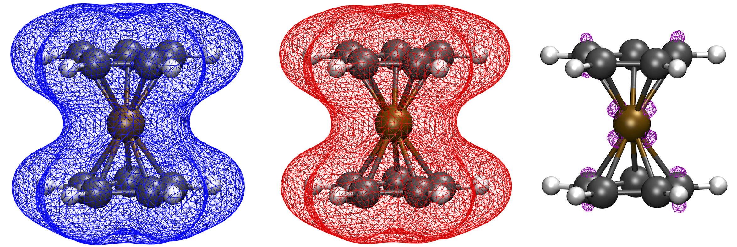
Example: Vertical ionization of Cobaltocene
An example might be to create a difference density plot between two redox states of a molecule. This can only cleanly be done for a vertical redox process.
from ash import *
import shutil

string="""
Co       6.344947000     -1.560817000      5.954256000
C        6.026452000     -0.546182000      7.802276000
C        5.793563000     -1.965872000      7.908267000
C        7.027412000     -2.657637000      7.660083000
C        7.976024000     -1.681400000      7.254253000
C        7.360141000     -0.371346000      7.359546000
H        5.287260000      0.234934000      7.955977000
H        4.853677000     -2.430623000      8.196105000
H        7.174908000     -3.733662000      7.680248000
H        7.845323000      0.573837000      7.130600000
C        7.003675000     -1.909758000      4.002507000
C        6.025582000     -2.892708000      4.310293000
C        4.831240000     -2.191536000      4.690416000
C        5.029751000     -0.780020000      4.468693000
C        6.380790000     -0.601338000      4.083942000
H        8.038293000     -2.097559000      3.727053000
H        6.179063000     -3.967316000      4.350882000
H        3.905308000     -2.652860000      5.025216000
H        6.875603000      0.346060000      3.887076000
H        4.297348000      0.002948000      4.644348000
H        8.999375000     -1.871686000      6.940915000
"""

#Defining fragment for redox reaction
Co_neut=Fragment(coordsstring=string, charge=0, mult=2)
Co_ox=Fragment(coordsstring=string, charge=1, mult=1)
label="Cocene_"+'_'
#Defining QM theory as ORCA here
qm=ORCATheory(orcasimpleinput="! BP86 def2-SVP tightscf notrah")

#Run neutral species with ORCA
e_neut=Singlepoint(theory=qm, fragment=Co_neut)
shutil.copyfile(qm.filename+'.gbw', label+"neut.gbw") # Copy GBW file
#Run orca_plot to request electron density creation from ORCA gbw file
run_orca_plot(label+"neut.gbw", "density", gridvalue=80)

#Run oxidized species with ORCA
e_ox=Singlepoint(theory=qm, fragment=Co_ox)
shutil.copyfile(qm.filename+'.gbw', label+"ox.gbw")  # Copy GBW file
#Run orca_plot to request electron density creation from ORCA gbw file
run_orca_plot(label+"ox.gbw", "density", gridvalue=80)

#Read Cubefiles from disk.
neut_cube_data = read_cube(label+"neut.eldens.cube")
ox_cube_data = read_cube(label+"ox.eldens.cube")
#Write out difference density as a Cubefile
write_cube_diff(neut_cube_data, ox_cube_data, label+"diffence_density.cube")
The script will output the files Cocene_neut.eldens.cube and Cocene_ox.eldens.cube that are here generated by orca_plot. The file Cocene_diffence_density.cube is generated by write_cube_diff.
Various analysis tools
CM5 charges can be calculated using the calc_cm5 function. This function requires the atomic numbers (list), coordinates (numpy array) and Hirschfeld charges (list) of the system:
def calc_cm5(atomicNumbers, coords, hirschfeldcharges):
Functions to calculate J-couplings according to Yamaguchi, Bencini or Noodleman formulas. All functions requires the energy of the high-spin and broken-symmetry energy.
#Yamaguchi equation also requires the <S^2> values of the high-spin and BS state.
def Jcoupling_Yamaguchi(HSenergy,BSenergy,HS_S2,BS_S2):
#The Bencini equation (strong-interaction limit, i.e. bond-formation) requires the maximum spin of the system.
def Jcoupling_Bencini(HSenergy,BSenergy,smax):
#The Noodleman equation (weak-interaction limit) also requires the maximum spin of the system.
def Jcoupling_Noodleman(HSenergy,BSenergy,smax):
NOCV analysis
NOCV analysis can be performed in ASH in 2 different ways: NOCV_density_ORCA or NOCV_Multiwfn
NOCV_density_ORCA calls on ORCA to perform the NOCV and ETS-NOCV. Note that the functionality is more complete in ORCA 6.1 and now available for the open-shell case.
Warning: The function below has not been tested with ORCA 6.1:
def NOCV_density_ORCA(fragment_AB=None, fragment_A=None, fragment_B=None, theory=None, griddensity=80,
                            NOCV=True, num_nocv_pairs=5, keep_all_orbital_cube_files=False,
                            make_cube_files=True):
The NOCV_Multiwfn function calls on Multiwfn to perform the NOCV and ETS-NOCV. The disadvantage is that the energy decomposition analysis is approximate as full ETS method is not performed.
def NOCV_Multiwfn(fragment_AB=None, fragment_A=None, fragment_B=None, theory=None, gridlevel=2, openshell=False,
                            num_nocv_pairs=5, make_cube_files=True, numcores=1, fockmatrix_approximation="ETS"):
Various ORCA-specific analysis tools
Read/write Fock matrix from/to ORCA outputfile.
# Convert Fock matrix into ORCA-format for printing. Returns string
def get_Fock_matrix_ORCA_format(Fock):
# Read Fock matrix from ORCA outputfile. Returns 2 numpy arrays (alpha and beta)
def read_Fock_matrix_from_ORCA(file):
# Write Fock matrix to disk as a dummy ORCA outputfile. Can be used by Multiwfn
def write_Fock_matrix_ORCA_format(outputfile, Fock_a=None,Fock_b=None, openshell=False):
Create difference density for 2 calculations differing in either fragment or theory-level. Theory level has to be ORCATheory. Difference density is written to disk as a Cube-file.
#Create difference density for 2 calculations differing in either fragment or theory-level
def difference_density_ORCA(fragment_A=None, fragment_B=None, theory_A=None, theory_B=None,
    griddensity=80, cubefilename='difference_density'):
Density sensitivity metric
A common problem in computational chemistry is DFT-method sensitivity and this is a particular problem in transition metal chemistry. In addition to energies changing there are cases where there are non-negligible changes in the electron density. Martin-Fernández and Harvey proposed an interesting normalized density sensitivity metric in 2021: see article
ASH has an implementation of this metric that allows one to easily check whether a particular molecule or system suffers from density sensitivity which would generally suggest that any DFT calculation on such a system should be carefully evaluated.
The ASH function density_sensitivity_metric performs DFT calculations of a system (an input fragment) with 2 different functionals, first in a regular self-consistent way, and then using the density of the second functional to calculate the energy with the former. Since modifying the HF Exchange frequently is the source of the most sensitivity, we choose 2 functionals with different amount of HF Exchange. Martin-Fernández and Harvey chose in their paper to use B3LYP with either 20 % or 25 % HF exchange. The ASH function allows one to choose a different hybrid functional form (e.g. PBE0) as well as changing the 2 HF Exchange percentages used. The function is hard-coded to perform these calculations using ORCA (ORCA must be in the environment PATH).
After the calculations are done we derive an energy-change due to density, E_D, and the energy-change due to functional, E_F, then the eps_D metric and finally the S_rho metric.
def density_sensitivity_metric(fragment=None, functional="B3LYP", basis="def2-TZVP", percentages=[0.20,0.25], numcores=1):
Example below shows how the metric is evaluated on 2 simple molecule using B3LYP functional, varying the HF exchange from 20 % to 25 % (as used in the paper).
from ash import *

#Molecules
H2O=Fragment(databasefile="h2o", charge=0, mult=1)
FeCO5=Fragment(xyzfile="feco5.xyz", charge=0, mult=1)

print("Calculating density_sensitivity_metric for H2O")
density_sensitivity_metric(fragment=H2O, functional="B3LYP/G", basis="def2-TZVP", percentages=[0.20, 0.25], numcores=4)
print("Calculating density_sensitivity_metric for Fe(CO)5")
density_sensitivity_metric(fragment=FeCO5, functional="B3LYP/G", basis="def2-TZVP", percentages=[0.20, 0.25], numcores=4)
This results in the output:

# For H2O

Density sensitivity metrics
------------------------------
delta_E: -25.661 kcal/mol
delta_E_F: -25.675  kcal/mol
delta_E_D:   0.014  kcal/mol
eps_D:   0.054 %
S_rho:    2.15

# For Fe(CO)5

Density sensitivity metrics
------------------------------
delta_E: -284.224 kcal/mol
delta_E_F: -284.685  kcal/mol
delta_E_D:   0.461  kcal/mol
eps_D:   0.162 %
S_rho:    6.49
As the results reveal there is clearly a much larger density sensitivity associated with the organometallic Fe(CO)5 compared to a plain water molecule, both according to the normalized S_rho metric, the eps_D metric and the delta_E_D metric.
As discussed in the original article, molecules can be roughly grouped into categories of density sensitivity based on the metrics above. Note that some of the metrics will be more sensitive to the precise protocol used (i.e. functional and HF exchange amounts used).
group |
delta_E_D |
eps_D (%) |
S_rho |
examples |
|---|---|---|---|---|
less sensitive |
<0.5 |
<0.150 |
<5.0 |
alkanes |
sensitive |
0.5-2.0 |
0.15-0.20 |
4.0-8.0 |
TM complexes |
extremely sensitive |
>3.5 |
>0.20 |
>8.5 |
FeMoco |