Hybrid Theory
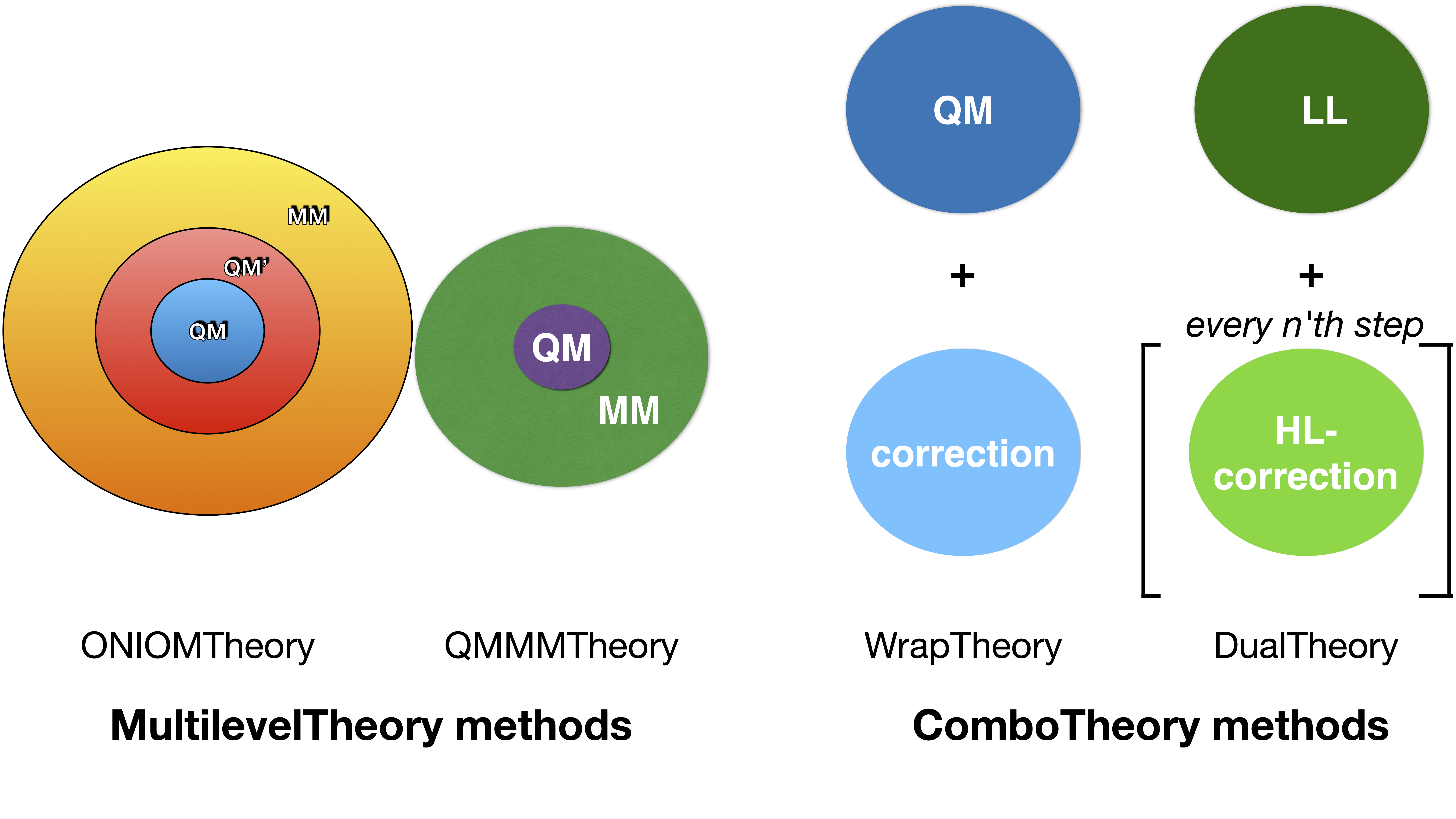
Hybrid Theories in ASH are theories that combine multiple theory objects to give some kind of combined theory description of the system. The different theories might be used for different parts of the system, then called Multilevel Theory methods (e.g. QMMMTheory or ONIOMTheory) or on the same part of the system, then called ComboTheory (examples are WrapTheory and DualTheory)
The strength of performing hybrid calculations in ASH is that in principle any level of theory in any QM or MM program interface can be combined with any other level of theory in any other QM or MM program interface to perform these hybrid-theory calculations.
Multilevel Theory Methods
QM/MM
The QMMMTheory class in ASH (QM/MM Theory) is a special type of a multilevel method where 1 single QMTheory is combined with 1 single MMTheory (usually OpenMMTheory, see OpenMM interface) to describe different parts of the system. QM/MM as a method is typically used when the system can naturally be divided up into a local important part (described by a QM method) and an environment part (described by a classical MM method). The coupling between QM and MM system is usually performed using electrostatic embedding. QM/MM is typically described as an additive energy expression:
where \(E_{QM}\) is the QM-energy of the QM-region, \(E_{MM}\) is the MM-energy of the MM-region and \(E_{coupling}\) is the interaction between the QM and MM region. The coupling terms account for electrostatic, vdW and covalent (bonded) interactions between the QM and MM regions and can be done using mechanical embedding, electrostatic embedding or polarized embedding (not yet in ASH). See QM/MM Theory for information on how to perform QM/MM calculations in ASH.
An alternative to the additive QM/MM expression is the subtractive ONIOM expression, here shown as a 2-layer ONIOM description:
2-layer ONIOM
The ONIOM method requires a low-level theory energy evaluation for the full system, a high-level theory (HL) calculation of the important part of the system and a low-level theory (LL) calculation of the environment part of the system. ONIOM is an interesting alternative to QM/MM because the low-level theory does not have to be an MM theory but can be a lower-level QM theory (e.g. semi-empirical QM or a cheap DFT description). See ONIOM for information on how to perform ONIOM calculations in ASH.
ComboTheory methods
ComboTheory methods are hybrid methods that unlike MultiLevelTheory methods don't partition the system into regions and , but describe the same system using multiple theories. WrapTheory is the most versatile version of this class of hybrid methods.
WrapTheory
WrapTheory is an ASH Theory class that wraps 2 or more different theory objects to get a combined theory description. An example would be where the energy and gradient from each theory is completely additive:
However, WrapTheory also supports arbitrary summation or subtraction of different theories:
A WrapTheory object can be used for geometry optimizations, surface scans, NEB calculations, molecular dynamics etc. As long as all theory components of the WrapTheory object are capable of producing an energy and gradient, then these job-types will automatically work with a WrapTheory object.
class WrapTheory:
    """ASH WrapTheory theory.
    Combines multiple theories to give a modified energy and modified gradient
    """
    def __init__(self, theories=None, theory1=None, theory2=None, printlevel=2, label=None,
                theory1_atoms=None, theory2_atoms=None, theory3_atoms=None,
                theory_operators=None):

    def run(self, current_coords=None, current_MM_coords=None, MMcharges=None, qm_elems=None, mm_elems=None,
    elems=None, Grad=False, PC=False, numcores=None, restart=False, label=None,
    charge=None, mult=None):
WrapTheory was initially created for the purpose of allowing one to combine a regular theory-level with some kind of correction (both energy and gradient) from another source. But the WrapTheory construct is nowadays even more versatile.
To use, one first defines 2 or more theory objects, combines them into a list and gives them to the theories keyword of WrapTheory (alternatively one can use theory1 and theory2 keywords).
Below we combine 2 objects but any number of objects can in principle be combined.
#Definition of some theories (here some dummynames are used)
t1 = SomeTheory()
t2 = OtherTheory()

# Wrapping of theories into a WrapTheory object
wrap = WrapTheory(theories=[t1,t2])
By default, energies and gradients are summed together (assuming complete additivity of the energy expressions). However, this behaviour can be changed by the theory_operators keyword. Below we change this so that the energy (and gradient) from the first theory is summed (used) but the second energy (and gradient) is subtracted.
Obviously such a hybrid method would only make sense for very specific theories (e.g. when correcting for double-counting of interations).
#Definition of theories
t1 = SomeTheory()
t2 = OtherTheory()

# Wrapping of theories in a sum+subtractive fashion
WrapTheory(theories=[t1,t2], theory_operators=['+','-'])
Also by default, the run-method of the WrapTheory object will request a calculation of the whole system for all theories. This can be changed by specifying the atom indices of the system for each theory. Below, we define a WrapTheory of 3 theories, and an energy expression where the first 2 theories are summed but the third is subtracted, and where Theory2 and Theory3 are only applied to a specific region of the system (atoms 3,4 and 5).
frag = Fragment(databasefile="acetone.xyz")

#Definition of theories
t1 = SomeTheory()
t2 = OtherTheory()
t3 = SomeOtherTheory()

# Wrapping of theories
WrapTheory(theories=[t1,t2,t3], theory_operators=['+','+','-'],
        theory1_atoms=frag.allatoms, theory2_atoms=[3,4,5], theory3_atoms=[3,4,5])
Note
The region of atoms specified by theory2_atoms and theory3_atoms should be whole molecules in general. If this region-definition crosses a covalent boundary then WrapTheory may not be the most suitable hybrid theory and better to use ONIOMTheory instead where linkatoms are automatically applied for covalent boundaries.
DFT+dispersion correction example:
Originally WrapTheory was created to allow one to easily add an additive dispersion correction using DFTD4Theory (see Helper-programs interfaces) to a regular DFT calculation (without dispersion).
This can be accomplished like below:
from ash import *

#Glycine fragment from database
frag = Fragment(databasefile="glycine.xyz")

#PBE/def2-SVP via ORCA (no dispersion correction)
orca = ORCATheory(orcasimpleinput="! PBE def2-SVP tightscf")
#DFTD4 dispersion correction using DFTD4 library
dftd4 = DFTD4Theory(functional="PBE")
#Combining the two theories using WrapTheory
dft_plus_dftd4_theory = WrapTheory(theories=[orca,dftd4])

#Calling the Optimizer function using the WrapTheory object as theory
Optimizer(theory=dft_plus_dftd4_theory, fragment=frag)
WrapTheory can be used for many other purposes, one would simply have to make sure that the theories used are compatible and that the combined theory-description does not result in double-counting of any similar physical energy terms. A regular DFT calculation (barely describes dispersion) + an atom pairwise dispersion correction (DFT-D4) is a good example of where the 2 theories are completely additive.
Composite DFT scheme example:
Composite methods such as r2SCAN-3c is another example where the energy of the method is a sum of 3 different contributions: A regular DFT-energy, a dispersion correction and a gCP (geometric counterpoise) correction.
A WrapTheory object can easily be created that defines r2SCAN-3c in this way.
See DFTD4 and gCP sections in Helper-programs interfaces for more information on the dispersion and gcp corrections.
from ash import *

#Acetone fragment from database
frag = Fragment(databasefile="acetone.xyz")

#r2SCAN/def2-mTZVPP via ORCA
orca_r2scan = ORCATheory(orcasimpleinput="! r2SCAN def2-mTZVPP def2-mTZVPP/J printbasis tightscf noautostart")
# gcp correction
gcp_corr = gcpTheory(functional="r2SCAN-3c", printlevel=3)
# D4 correction
d4_corr = DFTD4Theory(functional="r2SCAN-3c", printlevel=3)

#Combining the 3 theories using WrapTheory
r2scan3c = WrapTheory(theories=[orca_r2scan, gcp_corr,d4_corr])

#Calling the Optimizer function using the WrapTheory object as theory
Optimizer(theory=r2scan3c, fragment=frag)
Delta machine-learning correction example:
A \(\Delta\)-ML correction would be another example where WrapTheory would be convenient for combining Theory-levels.
See Machine learning in ASH on how to define and train ML-models.
from ash import *

#Glycine fragment from database
frag = Fragment(databasefile="glycine.xyz")

#PBE/def2-SVP via ORCA (no dispersion correction)
orca = ORCATheory(orcasimpleinput="! PBE def2-SVP tightscf")
# A pre-trained machine-learning correction (delta-ML)
ml = MACETheory(model_file="deltaML.model") #
#Combining the two theories using WrapTheory
dft_plus_deltaml = WrapTheory(theories=[orca,ml])

#Calling the Optimizer function using the WrapTheory object as theory
Optimizer(theory=dft_plus_deltaml, fragment=frag)
Combining QM/MM, ML in an additive+subtractive combination for different regions:
A more complex hybrid theory involves combining an electrostatic-embedding QMMMTheory object (where QM and MM-regions are already defined) with a general machine-learning model (ML). The ML-theory might furthermore only be applied to certain atoms such as the QM-region (see use of theory2_atoms below). In order to avoid double-counting of the QM-region we have to subtract the QM-method energy of the QM-region.
This can all be accomplished using WrapTheory by utilizing theory_operators=['+','+','-'] and theory1_atoms, theory2_atoms and theory3_atoms keywords.
Note
The region of atoms specified by theory2_atoms and theory3_atoms should be whole molecules in general. If this region-definition crosses a covalent boundary then WrapTheory may not be the most suitable hybrid theory and better to use ONIOMTheory instead where linkatoms are automatically applied for covalent boundaries.
from ash import *


# H2O...MeOH fragment defined. Reading XYZ file
frag = Fragment(xyzfile=f"h2o_MeOH.xyz")
pdbfile="h2o_MeOH.pdb"
# Specifying the QM atoms (3-8) by atom indices (MeOH). The other atoms (0,1,2) is the H2O and MM.
# IMPORTANT: atom indices begin at 0.
qmatoms=[3,4,5,6,7,8]

# QM
qm = xTBTheory()
# MM: OpenMMTheory using XML-file
MMpart = OpenMMTheory(xmlfiles=[f"MeOH_H2O-sigma.xml"], pdbfile=pdbfile, autoconstraints=None, rigidwater=False)

# Creating QM/MM object
QMMMobject = QMMMTheory(fragment=frag, qm_theory=qm, mm_theory=MMpart, qmatoms=qmatoms,
                        embedding='Elstat', qm_charge=0, qm_mult=1)

ml = MACETheory(model_file="../MACE-omol-0-extra-large-1024.model")

wrap = WrapTheory(theories=[QMMMobject,ml,qm], theory_operators=['+','+','-'], printlevel=3,
    theory1_atoms=frag.allatoms, theory2_atoms=qmatoms, theory3_atoms=qmatoms)

# Single-point energy calculation of QM/MM object
result = Singlepoint(theory=wrap, fragment=frag, charge=0, mult=1, Grad=True)
DualTheory
DualTheory is an experimental ASH Theory that combines two different theory objects, e.g. a low-level QM theory and a high-level QM theory in a specific way in order to speed up an otherwise expensive high-level calculation. This only makes sense for an expensive multi-iteration job where the Theory object is called multiple times, e.g. a geometry optimization or NEB calculation (not a single-point calculation).
The idea is to approximate the accurate high-level potential energy surface description by a low-level potential energy surface desciption + a correction derived from the high-level theory. If the correction is calculated in every step (of e.g. a geometry optimization) there is no advantage (in fact more expensive) to using a DualTheory description. However, if the high-level correction is only occasionally calculated then it possible to cut down on the number of expensive high-level energy+gradient calculations required.
Both energy and the gradient (required for optimizations and NEB calculations) can be corrected.
Currently the only available correction option is: "Difference" which features a naive energy/gradient difference correction. The update_freq keyword controls the interval between corrections. To use a Dualtheory one needs to give valid ASH Theory objects to the theory1 and theory2 keywords where theory1 is assumed to be the low-level theory (called each time) while theory2 is the high-level theory ( called only when the high-level correction should be updated according to the value of update_freq).
class DualTheory:
    """ASH DualTheory theory.
    Combines two theory levels to give a modified energy and modified gradient
    """
    def __init__(self, theory1=None, theory2=None, printlevel=2, label=None, correctiontype="Difference", update_freq=5, numcores=1):
Geometry optimization example using GFN1-xTB and DFT:
from ash import *

numcores=1
frag=Fragment(xyzfile="react.xyz", charge=0, mult=1)

#Defining theory levels
xtb = xTBTheory(xtbmethod="GFN1", numcores=numcores)
orca = ORCATheory(orcasimpleinput="!r2scan-3c tightscf CPCM", numcores=numcores)

#Creating DualTheory object:
#theory1 is the cheaper low-level theory called in each step, theory2 is the less-called high-level theory
dualcalc = DualTheory(theory1=xtb, theory2=orca, update_freq=15)

#Calling the Optimizer function using the DualTheory object
Optimizer(theory=dualcalc, fragment=frag, maxiter=250)
A nudged elastic band job example using GFN1-xTB and DFT:
from ash import *

numcores=1

#Fragment for an SN2 reaction
Reactant=Fragment(xyzfile="react.xyz", charge=-1, mult=1)
Product=Fragment(xyzfile="prod.xyz",charge=-1, mult=1)

#Defining individual theory levels
xtb = xTBTheory(numcores=numcores)
orca = ORCATheory(orcasimpleinput="!r2scan-3c tightscf CPCM", numcores=numcores)

#Creating DualTheory object:
#theory1 is the cheaper low-level theory called in each step, theory2 is the less-called high-level theory
dualcalc = DualTheory(theory1=xtb, theory2=orca, update_freq=5)

#Calling the NEB job function using the DualTheory object
NEB(reactant=Reactant, product=Product, theory=dualcalc, images=12, printlevel=0, maxiter=200)