Surface Scan

Potential Energy Surfaces can be conveniently scanned in ASH using the calc_surface function . This function performs unrelaxed and relaxed scans and can utilize either the geomeTRIC Optimizer, the DL-FIND Optimizer or the ASH built-in Cartesian optimizer (see Geometry optimization) to carry out the constrained optimizations needed for the scans.

Surface scans explore the potential energy surface by gradually changing and freezing one or more suitable geometric coordinates while optimizing all other geometric coordinates. The calc_surface has been rewritten and now supports any number of scan variables, meaning, 1D, 2D and even 3D surface scans are possible (and beyond, if really required).

While surface scans can also be used to approximate minimum energy paths between minima and locate approximate saddlepoints ("Transition states"), it is strongly advised to instead use the Nudged Elastic Band for this purpose.

def calc_surface(
    fragment=None, theory=None, charge=None, mult=None, optimizer='geometric',
    scantype='UNRELAXED', resultfile='surface_results.txt',
    keepoutputfiles=True, keepmofiles=False,
    runmode='serial', coordsystem='dlc', maxiter=250,
    NumGrad=False, extraconstraints=None,
    convergence_setting=None, conv_criteria=None,
    subfrctor=1, force_noPBC=False,
    numcores=1, ActiveRegion=False, actatoms=None,
    PBC_format_option="CIF",
    # ---- New N-dimensional interface ----
    RC_list=None,
    # ---- Legacy 1D/2D interface (kept for backward compatibility) ----
    RC1_range=None, RC1_type=None, RC1_indices=None,
    RC2_range=None, RC2_type=None, RC2_indices=None,
):

Keyword	Type	Default value	Details
theory	ASH THeory	None	An ASH Theory.
fragment	ASH Fragment	None	An ASH fragment.
scantype	string	'Unrelaxed'	What type of scan to perform. Options: 'Unrelaxed' and 'Relaxed'
RC_list	list	None	New syntax: A list of dictionaries that define the reaction coordinates (RC)..
RC1_indices/RC2_indices	list of integers	None	Old syntax: List of atom indices defining Reaction coordinate(RC) 1 or 2.
RC1_type/RC2_type	string	None	Old syntax: String indicating the type of reaction coordinate (either RC1 or RC2). Option: 'bond', 'angle', 'dihedral'
RC1_range/RC2_range	list of floats	None	Old syntax: List of number indicating the range of values to scan for RC1 or RC2. Example: [2.0,2.2,0.01] indicates scan value from 2.0 to 2.2 in 0.01 increments.
runmode	string	'serial'	Whether to run calculations in serial or parallel. Options: 'serial', 'parallel'.
resultfile	string	'surface_results.txt'	Change name of the results-file.
extraconstraints	Dict	None	Dictionary of additional constraints to apply during optimization. See Geometry optimization.
coordsystem	string	'tric'	Which coordinate system to use during optimization. Options: 'tric', 'hdlc', 'dlc', 'prim', 'cart' Default: 'tric' (TRIC: translation+rotation internal coordinates), for an active region 'hdlc' is used instead. See Geometry optimization.
maxiter	integer	100	Maximum number of optimization iterations before giving up (for scantype='Relaxed').
convergence_setting	string	None.	Specifies the type of convergence criteria for Optimizer. Options: 'ORCA', 'Chemshell', 'ORCA_TIGHT', 'GAU', 'GAU_TIGHT', 'GAU_VERYTIGHT', 'SuperLoose'. See Convergence section for details.
ActiveRegion	Boolean	False	Whether to use an Active Region during the optimization. This requires setting the number of active atoms (actatoms list) below.
actatoms	list	None	List of atom indices that are active during the optimization job. All other atoms are frozen.
keepoutputfiles	Boolean	False	Whether to keep outputfile for each surfacepoint from QM code or not.
keepmofiles	Boolean	False	Whether to keep MO-files for each surfacepoint from QM code or not. Only works for ORCATheory.
read_mofiles	Boolean	False	Whether to read MO-files (from mofilesdir) for each surfacepoint or not.
mofilesdir	string	None	Path to the directory containing MO-files. Use with read_mofiles=True option.
charge	integer	None	Optional specification of the charge of the system (if QM) if the information is not present in the fragment.
mult	integer	None	Optional specification of the spin multiplicity of the system (if QM) if the information is not present in the fragment.

Parallelization

Surface scans can be parallelized in one of 2 ways. Either you run :

i) each surfacepoint one after the other (runmode="serial", this is default) (using the optimized geometry of the previous surfacepoint and possible MOs as well) while parallelizing the Theory-level of each surfacepoint. This approach does not parallelize as well (QM calculations have limitations regardign parallelization) but has the advantage of likely avoiding convergence issues or falling into local minima.

This strategy is the simplest to start with.

ii) (runmode="parallel" and select numcores) Here surfacepoints are run in parallel and independently of each other. Here we can utilize all X available CPU cores on the computer and run X surfacepoint calculations at the same time. We typically want to turn off any Theory parallelization for this scenario (almost never desired) by setting numcores in Theory object to be 1. If you have many surfacepoints, this might be the most efficient parallelization strategy. A disadvantage is that convergence can be affected since scanpoints with geometries far from the initial structure, could struggle to converge and could fall into local minima.

How to use

The calc_surface function always takes a Fragment and Theory object as input. The type of scan should be specified via scantype ('Unrelaxed' or 'Relaxed') and runmode should be chosen according to the parallelization strategy (see above).

We then need to define the reaction coordinate.

New syntax: Defining Reaction Coordinates via RC_list It is recommended to use the newer syntax of using the RC_list keyword. Here we define a list of dictionaries that define the desired Reaction-Coordinates

# Defining RCs via list of dictionaries:
RC_list=[{'type': 'dihedral',  'indices': [[0,1,2,3]], 'range': [-180, 180, 10]},
          {'type': 'angle',  'indices': [[1,0,2]], 'range': [180, 100, -10]}
          {'type': 'bond',  'indices': [[1,0]], 'range': [1.1, 1.5, 10]}])

This general syntax allows any number of RCs to be defined, meaning we can define 1D, 2D, 3D surface scans and even beyond that.

Old syntax: Defining Reaction Coordinates via RCX_type/RCX_indices/RCX_range keywords

The older syntax is only available for either 1 or 2 reaction coordinates. One specifies RC1_type, RC1_range and RC1_indices (and also RC2 versions if 2 reaction coordinates are wanted).

• The RC1_type/RC2_type keyword can be: 'bond', 'angle' or 'dihedral' .

• The RC1_indices/RC2_indices keyword defines the atom indices for the bond/angle/dihedral. Note: ASH counts from zero.

• The RC1_range/RC2_range keyword species the start coordinate, end coordinate and the stepsize (Å units for bonds, ° for angles/dihedrals).

The old syntax is only kept for backward compatibility and will probably be removed at some point.

Result file The resultfile keyword should be used to specify the name of the file that contains the results of the scan ( format: coord1 coord2 coord3... energy). This file can be used to restart an incomplete/failed scan and to plot the final surface. If ASH finds this file in the same dir as the script, it will read the data and skip unneeded calculations. By default it is named: 'surface_results.txt'

calc_surface returns an ASH Results object that contains a dictionary of total energies for each surface point. The key is a tuple of coordinate values and the value is the energy, i.e. (RC1value,RC2value) : energy

1D scan:

Here scanning an angle (defined by atom indices 1,0,2 and scanning from 180° to 110 by taking decreasing steps of 10°).

results = calc_surface(fragment=frag, theory=ORCAcalc, scantype='Unrelaxed',
      resultfile='surface_results.txt',
      runmode='serial', RC_list=[{'type': 'angle',  'indices': [[1,0,2]], 'range': [180, 110, -10]}],
      keepoutputfiles=True, surfacedictionary = results.surfacepoints

2D scan:

If 2 dictionaries are defined in RC_list (or alternatively in the old syntax: if both RC1 and RC2 keywords are provided) then a 2D scan will be calculated. Below we scan both a bond(distance) between 2.0 and 2.2 Å (0.01 Å step) for atom-pairs [0,1] and [0,2]. and the angle (between atoms 1,0,2) from 180° to 100°.

As can be seen it is possible to have each RC apply to multiple sets of atom indices by specifying a list of lists. In this 2D scan example , the first RC (bond/distance) is applied to both atoms [0,1] as well as [0,2]. This typically makes sense when one wants to preserve the symmetry of a system e.g. this might apply to the O-H bonds in H2O.

results = calc_surface(fragment=frag, theory=ORCAcalc, scantype='Unrelaxed', resultfile='surface_results.txt',
          runmode='serial',
          RC_list=[{'type': 'bond',  'indices': [[0,1],[0,2]], 'range': [2.0, 2.2, 0.01]},
                   {'type': 'angle',  'indices': [[1,0,2]], 'range': [180, 100, -10]}],
                    keepoutputfiles=True)

Choosing between geometry optimizers

While the geomeTRICOptimizer is currently the default optimizer and works generally well, there are cases where other optimizers might be preferred. This might be the case if the geomeTRIC optimizer overhead becomes a considerable part of the surface-scan, and the surface-scan contains many points. Another reason for switching between optimizers might be if the constrained optimization has trouble converging, then switching to a different optimizer might help.

If you are using a Theory level that has very fast execution speed: e.g. a forcefield via OpenMMTheory, a machine-learning potential via PyTorch or perhaps a semiempirical method like GFN2-xTB, then the energy+gradient calculations calculated by the Theory object may be so fast that the bottleneck of the surfacescans may be the set-up and run of the geometry optimization algorithms themselves.

Use of the DL-FIND optimizer can be an attractive option in such cases, being a very fast and robust optimizer, written in Fortran and with very low overhead. DL-FIND implements hard constraints and features HDLC internal coordinates. Another option is the ASH built-in Cartesian optimizer. Because it avoids the overhead of internal coordinate transformations, it can be very fast for small systems and scans with many points. It features soft constraints instead of hard constraints but often works well.

Telling calc_surface to use DL-FIND instead is easy and scan-variables and additional constraints are handled in the same manner.

Alternatively,

Do note that certain calc_surface keywords may be specific to each optimizer.

Surface scan using the geomeTRIC optimizer

results = calc_surface(fragment=frag, theory=ORCAcalc, scantype='Relaxed', optimizer="geometric",
          RC_list=[{'type': 'bond',  'indices': [[0,1],[0,2]], 'range': [2.0, 2.2, 0.01]},
                   {'type': 'angle',  'indices': [[1,0,2]], 'range': [180, 100, -10]}])

geomeTRICOptimizer-specific options in calc_surface:

• coordsystem (for geomeTRICOptimizer, default: 'dlc'. Other options: 'hdlc' and 'tric')

• maxiter (for geomeTRICOptimizer,default : 50)

• convergence_setting (for geomeTRICOptimizer, same syntax as in geomeTRICOptimizer)

Surface scan using the DL-FIND optimizer

results = calc_surface(fragment=frag, theory=ORCAcalc, scantype='Relaxed', optimizer="dlfind",
          RC_list=[{'type': 'bond',  'indices': [[0,1],[0,2]], 'range': [2.0, 2.2, 0.01]},
                   {'type': 'angle',  'indices': [[1,0,2]], 'range': [180, 100, -10]}])

In order to use special optimization settings for the DLFIND Optimizer, there is an option to first create a DLFINDOptimizer_class object, then provide that object to calc_surface.

# Create a DLFIND Optimizer object with special settings
dlfind_optimizer = DLFIND_optimizerClass(theory=theory, fragment=fragment,
                    maxcycle=300, tolerance=4.5E-4, tolerance_e=1E-6,
                    constraints={'bond':[0,1]})
# Provide the optimizer object to calc_surface
results = calc_surface(fragment=frag, theory=ORCAcalc, scantype='Relaxed', optimizer=dlfind_optimizer,
          RC_list=[{'type': 'bond',  'indices': [[0,1],[0,2]], 'range': [2.0, 2.2, 0.01]},
                   {'type': 'angle',  'indices': [[1,0,2]], 'range': [180, 100, -10]}])

Surface scan using the ASH Cartesian optimizer

The ASH Cart_optimizer is a built-in Cartesian optimizer that can be used for the constrained optimizations during the surface scan. It optimizes only in Cartesian coordinates (not internal coordinates) and may thus take more optimization steps than the other optimizers. However, it has the advantages of very low overhead (it avoids the overhead of internal coordinate transformations) and can be very fast for small systems and scans with many points. It uses soft constraints instead of hard constraints but this can be perfectly sufficient and the accuracy is tunable by modifying the force constants involved.

Using Cart_optimizer in calc_surface with default options:

results = calc_surface(fragment=frag, theory=ORCAcalc, scantype='Relaxed', optimizer="cartopt",
          RC_list=[{'type': 'bond',  'indices': [[0,1],[0,2]], 'range': [2.0, 2.2, 0.01]},
                   {'type': 'angle',  'indices': [[1,0,2]], 'range': [180, 100, -10]}])

In order to use special optimization settings for the ASH Cartesian Optimizer, one has to first create a Cart_optimizer_class object, then provide that object to calc_surface.

# Create a Cart_optimizer_class object with special settings
cart_optimizer = Cart_optimizer_class(step_algo="bfgs",maxiter=150, printlevel=1,
                  kf_bonds=10.0, kf_angles=10.0, kf_dihedrals=10.0)
# Provide the optimizer object to calc_surface
results = calc_surface(fragment=frag, theory=ORCAcalc, scantype='Relaxed', optimizer=cart_optimizer,
          RC_list=[{'type': 'bond',  'indices': [[0,1],[0,2]], 'range': [2.0, 2.2, 0.01]},
                   {'type': 'angle',  'indices': [[1,0,2]], 'range': [180, 100, -10]}])

Note: See Geometry optimization for discussion of the different optimizers: geomeTRIC, DL-FIND and Cart_optimizer.

Periodic boundary conditions

As the ASH interfaces to geomeTRIC, DL-FIND and Cart_optimizer can also optimize cell parameters, it is possible to perform geometry optimizations of both atom and lattice positions in a periodic system. This feature can be extended to constrained optimizations allowing surface scans via calc_surface to be carried out under PBCs. See Geometry optimization documentation for more information on the optimization aspect. This option is currently only available for the geomeTRIC Optimizer.

To enable PBC-based surface scans one simply needs to :

• create an ASH Fragment containing the Cartesian coordinates of the unitcell (can be an XYZ-file or something else).

• provide an ASH Theory object that has native support for PBCs (and PBC enabled) and provide cell vectors or cell dimensions to object.

• calc_surface will automatically recognize whether the Theory object has PBCs enabled.

See Periodic boundary conditions in ASH for information on what Theory objects are supported.

The PBC_format_option keyword can be used to specify the file format used for each surfacepoint that will be stored in the surface_pbcfiles directory. PBC_format_option takes options: 'CIF', 'XSF' or 'POSCAR' CIF-files and POSCAR file can be visualized in Chemcraft while XSF files can be visualized in VMD.

An example

from ash import *

numcores=1

#Create fragment from xyz-file
fragment=Fragment(xyzfile="system_unitcell.xyz", charge=0, mult=1)

#Periodic CP2KTheory definition with specified cell dimensions
qm = CP2KTheory(cp2k_bin_name="cp2k.psmp",parallelization='OMP',
    basis_method='XTB', xtb_type='GFN1',
    numcores=numcores, scf_maxiter=1500,
    periodic=True,cell_dimensions=[13.8,8.9,15.4,90,90,90],
    psolver='periodic', OT_preconditioner="FULL_SINGLE_INVERSE",
    eps_default=1e-12, stress_tensor=True)

# Scan using HDLC internal coordinates for the constrained optimizations
# NOTE: PBC_format_option: 'CIF', 'XSF', or 'POSCAR
results = calc_surface(fragment=fragment, theory=qm, scantype='relaxed',
    resultfile='surface_results.txt',
    runmode='serial',
    RC_list=[{'type': 'dihedral',  'indices': [[6,17,14,10]], 'range': [0,360,10]},
        {'type': 'dihedral',  'indices': [[51,62,59,55]], 'range': [0, 360, 10]}],
        coordsystem='hdlc', PBC_format_option="CIF")

Working with a previous scan from collection of XYZ files

If a surface scan has already been performed (by calc_surface or something else), it's possible to use the created XYZ-files and calculate single-point energies or optimizations for each surfacepoint with any level of theory.

def calc_surface_fromXYZ(xyzdir=None, theory=None, dimension=None, resultfile=None, scantype='Unrelaxed',runmode='serial',
                        coordsystem='dlc', maxiter=50, extraconstraints=None, convergence_setting=None, numcores=None,
                        RC_list=None, RC1_type=None, RC2_type=None, RC1_indices=None, RC2_indices=None,
                        keepoutputfiles=True, keepmofiles=False, read_mofiles=False, mofilesdir=None):
    """Calculate 1D/2D surface from XYZ files

    Args:
        xyzdir (str, optional): Path to directory with XYZ files. Defaults to None.
        theory (ASH theory, optional): ASH theory object. Defaults to None.
        dimension (int, optional): Dimension of surface. Defaults to None.
        resultfile (str, optional): Name of resultfile. Defaults to None.
        scantype (str, optional): Tyep of scan: 'Unrelaxed' or 'Relaxed' Defaults to 'Unrelaxed'.
        runmode (str, optional): Runmode: 'serial' or 'parallel'. Defaults to 'serial'.
        coordsystem (str, optional): Coordinate system for geomeTRICOptimizer. Defaults to 'dlc'.
        maxiter (int, optional): Max number of iterations for geomeTRICOptimizer. Defaults to 50.
        extraconstraints (dict, optional): Dictionary of constraints for geomeTRICOptimizer. Defaults to None.
        convergence_setting (str, optional): Convergence setting for geomeTRICOptimizer. Defaults to None.
        numcores (float, optional): Number of cores. Defaults to None.
        RC1_type (str, optional):  Reaction-coordinate type (bond,angle,dihedral). Defaults to None.
        RC2_type (str, optional): Reaction-coordinate type (bond,angle,dihedral). Defaults to None.
        RC1_indices (list, optional):  List of atom-indices involved for RC1. Defaults to None.
        RC2_indices (list, optional): List of atom-indices involved for RC2. Defaults to None.

    Returns:
        [type]: [description]
    """

We can use the calc_surface_fromXYZ function to read in previous XYZ-files (named like this: RC1_2.0-RC2_180.0.xyz for a 2D scan and like this: RC1_2.0.xyz for a 1D scan). These files should have been created from calc_surface already (present in surface_xyzfiles results directory). By providing a theory level object we can then easily perform single-point calculations for each surface point or alternatively relax the structures employing constraints. The results is a dictionary like before.

#Directory of XYZ files. Can be full path or relative path.
surfacedir = '/users/home/ragnarbj/Fe2S2Cl4/PES/Relaxed-Scan-test1/SP-DLPNOCC/surface_xyzfiles'

#Calculate surface from collection of XYZ files. Will read old surface-results.txt file if requested (resultfile="surface-results.txt")
#Unrelaxed single-point job
results = calc_surface_fromXYZ(xyzdir=surfacedir, scantype='Unrelaxed', theory=ORCAcalc, dimension=2,
            resultfile='surface_results.txt' )
surfacedictionary = results.surfacepoints

#Relaxed optimization job. A geometry optimization with constraints will be done for each point
#The RC1_type and RC1_indices (and RC2_type and RC2_indices for a 2D scan) also need to be provided
results = calc_surface_fromXYZ(xyzdir=surfacedir, scantype='Relaxed', theory=ORCAcalc, dimension=2,
                    resultfile='surface_results.txt',
                    coordsystem='dlc', maxiter=50, extraconstraints=None, convergence_setting=None,
                    RC_list=[{'type': 'bond',  'indices': [[0,1],[0,2]], 'range': [2.0, 2.2, 0.01]},
                    {'type': 'angle',  'indices': [[1,0,2]], 'range': [100, 150, 10]}],)
surfacedictionary = results.surfacepoints

Other options:

• keepoutputfiles=True (outputfile for each point is saved in a directory. Default True)

• keepmofiles=False (Boolean, MO-file for each point is saved in a directory. Default False)

• read_mofiles=False (Boolean: Read MO-files from directory if True. Default False.)

• mofilesdir=path (Directory path containing MO-files (GBW files if ORCA) )

• ActiveRegion= True/False

• actatoms=list (list of active atoms if doing relaxed scan)

Analyzing the surface (experimental)

The final result of the scan can be found in a textfile ('surface_results.txt' by default) or as a dictionary in the ASH Results object (returned by calc_surface and calc_surface_fromXYZ ).

ASH contains a function analyze_surface that attempts to automatically analyze the calculated energy surface and detect local and global minima as well as saddlepoint and maxima. This analysis should be exact for 1D scans but is more approximate for 2D and 3D surfaces (and beyond). Saddlepoint detection is hit-and-miss.

results = analyze_surface(resultfile='surface_results.txt', energy_unit='kcal/mol',
            tol=1e-6)

The function spits out a text output like below:

================================================================================
SURFACE ANALYSIS
================================================================================

MINIMA
--------------------------------------------------------------------------------
    65.0000    -80.0000      -16.7600375595 Eh        0.0000 kcal/mol  (global min)

MAXIMA
--------------------------------------------------------------------------------
   115.0000   -125.0000      -16.7578845482 Eh        2.6394 kcal/mol  (global max)
  -100.0000   -120.0000      -16.7595899788 Eh        1.5692 kcal/mol  (local max)

SADDLE POINTS
--------------------------------------------------------------------------------
    10.0000   -175.0000      -16.7609859067 Eh        0.6933 kcal/mol    (1-order SP)
  -125.0000   -175.0000      -16.7609600772 Eh        0.7095 kcal/mol    (1-order SP)
  -125.0000   -170.0000      -16.7609276133 Eh        0.7298 kcal/mol    (1-order SP)
  -105.0000   -175.0000      -16.7609271752 Eh        0.7301 kcal/mol    (1-order SP)

Additionally the results object from the function, contains a dictionary with the same data.

Warning

analyze_surface should be considered experimental.

Plotting

To plot the results, the dictionary can be given as input to some ASH plotting functions (based on Matplotlib). See Plotting) page.

The dictionary has the format: (coord1,coord2) : energy for a 2D scan and (coord1) : energy for a 1D scan where (coord1,coord2)/(coord1) is a tuple of floats and energy is the total energy as a float.

A dictionary using data from a previous job (stored e.g. in surface_results.txt) can be created via the read_surfacedict_from_file function:

Example

from ash import *

# Read in the results of a previous scan from file surface_results.txt into a dictionary
surfacedictionary = read_surfacedict_from_file("surface_results.txt")

#Plot a 1D scan:
reactionprofile_plot(surfacedictionary, finalunit='kcal/mol',label='Plotname', x_axislabel='Angle',
            y_axislabel='Energy', imageformat='png', RelativeEnergy=True, pointsize=40,
            scatter_linewidth=2, line_linewidth=1, color='blue')
#Plot a 2D scan:
contourplot(surfacedictionary, finalunit='kcal/mol',label="Plotname", interpolation='Cubic',
            x_axislabel='Bond (Å)', y_axislabel='Angle (°)')
# Plot a 3D scan (requires plotly)
volumeplot(surfacedictionary, x_axislabel='Bond length (Å)', y_axislabel='Angle (°)',
            z_axislabel='Dihedral (°)', colorbar_label='Energy', finalunit='kcal/mol',
            RelativeEnergy=True)

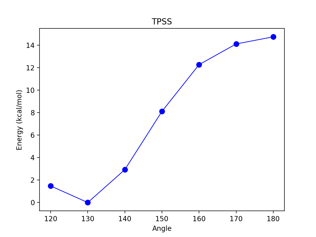
Figure 2. 1D Energy Surface scanning an angle of some molecule

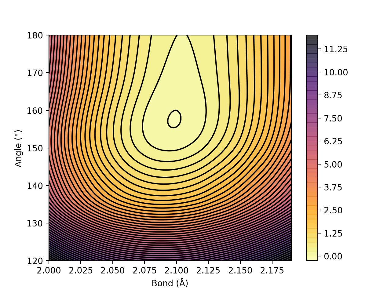
Figure 2. 2D Energy surface of FeS2 scanning both the Fe-S bond and the S-Fe-S angle. The Fe-S bond coordinate applies to both Fe-S bonds.

Figure 3. 3D energy surface of ethanol, scanning C-C bond length, <O-C-C> angle and <C-C-O-H torsion